Circular Features at Good Earth/Blood Run

Beyond Just Defining Lines

We looked at how circular archaeological features helped to define lines at Blood Run National Historic Landmark (NHL) in the last post. I also incorrectly located the NHL as 30 miles east of Lone Tree Farm; it’s actually 30 miles west of the Farm. As I told the friend who kindly pointed out that mistake, “I’m used to describing the location of the Farm relative to the NHL rather than the other way around.”

We really don’t know what function the linear archaeological features served at Blood Run or at the Farm, for that matter. Mainly, I just described the observations used to define the lines: landscape elements, LiDAR, patterns in artifact distribution, and alignments of circular archaeological features like mounds and cache pits. In this post we’ll look at the circular features a little closer and try to hit on some of the interpretations about what they were used for. The observations we’ll use to identify circular features will include: topography, rock outlines, soil patterns, and vegetation.

FIGURE 1---- A) Neighborhoods on LiDAR. B) Mounds in Neighborhood 4.

Both of these images are included in the previous post, but this time we’ll emphasize the circular features. The LiDAR landscape generated by the Iowa Office of the State Archaeologist (OSA) (Figure 1-A) has been modified to show the locations of the four “neighborhoods” of mounds in the main mound group at Blood Run. We’ll start with a look at mounds and cache pits in Neighborhood 4 and then cross the creek and go southwest along the terrace to look at patterns in Neighborhoods 1 and 2.

The large circles in Figure 1-B are mounds. Using the measurements produced during the surveys done by Lewis in the late 1880s, we can calculate a ratio that may relate to mound construction. Mounds in the northwest part of the group have a higher height (H)/base diameter (B) than the mounds in the southeastern area. This means that the mounds to the northwest stood higher than mounds in the southeast; that may be because the taller mounds are constructed of “rammed” earth whereas the shorter mounds are “soft” and didn’t resist erosion as well. There are stories of both types of construction encountered during salvage excavations in the “transition” zone. Some of the mounds that Lewis mapped have totally disappeared into the gravel pit operations, so of the 12 original mounds in that area, only 2 or 3 remained in 1980s when the salvage excavations were done. Although these mound interpretations are fairly speculative, the smaller circles mark some of the cache pits and those are somewhat easier in interpret.

FIGURE 2----Cache pits. A) 1980s photo of cache pit excavation in Neighborhood 4. B) Illustration in Good Earth visitor’s Center.

Several excavated cache pits are shown in Figure 2-A. The people working on excavating these circular features give some idea of the size of these smaller features. The mounds are topographic hills whereas the cache pits are smaller diameter holes that extend below ground. Also, in contrast to the limited digging done on the mounds, these cache pits were fairly completely excavated. Consequently, the record of artifacts within these features allows a pretty clear understanding of how they were used as storage pits (Figure 2-B). Often the pits were filled with refuse after the stored contents had been removed.

Figure 3---- A) Graph summarizing the relationship between cache pit size and number of artifacts. B) Map of cache pit trends in Neighborhood 4.

The artifacts found in the cache pits can be counted and as expected, the large pits have more artifacts than the smaller ones (Figure 3-A). However, there are four pits (marked by red and green stars, Figure 3-A and 3-B) that have more artifacts than predicted by the trend line. Three of those off-trend cache pits are located at the intersection of linear features trending southeast and northeast. This serves to reenforce the trends of linear features described in the previous post. But, topographic attributes like mounds and cache pits aren’t the only way that circular features find expression at Blood Run NHL.

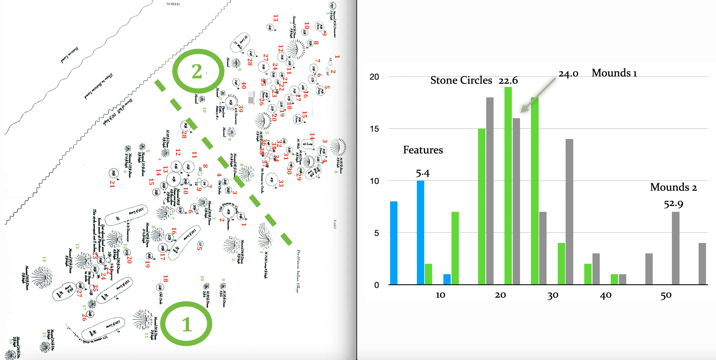
Figure 4----A) Pettigrew’s map of circular features in Neighborhoods 1 and 2. Red numbers count the rock circles and the green numbers count the mounds. B) Frequency diagram for diameters measured in feet.

To the southwest in Neighborhoods 1 and 2 (Figure 1-A), outlines of circles made of rocks were mapped by Pettigrew (Figure 4-A) back in the1880s even before Lewis formally measured the mounds. Those circular features have been thought to be “tepee rings” where the rocks supposedly held down the hide covering the outside of the dwelling. However, that interpretation has often been challenged by traditional knowledge keepers. In any case, the old 1880s maps of rock circles and mounds can be used to count the features and that exercise demonstrates some differences between Neighborhoods 1 and 2: Neighborhood 1 has 17 mounds and 27 rock circles, but Neighborhood 2 has only 10 mounds but has 40 circles.

The old maps also provide a way measure the diameters of the circular features and there are some distinct patterns in these size measurements. The diameters of the stone or rock circles are about the same as the diameters of the majority of the mounds (about 23 ft and 24 ft, Figure 4-B, green and gray, respectively). There’s another peak of mound diameters at about 53 ft and the cache pit diameters are much smaller at about 5 ft in diameter. Note that these numbers include the features in Neighborhood 4 as well as Neighborhoods 1 and 2.

FIGURE 5----A) Circular features surveyed by Lewis in Neighborhoods 1 and 2. B) Small circles on the floodplain of Blood Run Creek visible on high-resolution air photos (brown image in lower left) and satellite images (green image on right).

The map (Figure 5-A) prepared from survey measurements in the late 1880s by Lewis, shows the general pattern differences in Neighborhoods 1,2, and 3. There was an “Enclosure” mapped to the south of the railroad, but it’s no longer present. However, there does appear to be a circular arrangement of features (marked by the red circle, Figure 5-A) in Neighborhood 1 that sets it apart from Neighborhoods 2 and 3.

On the floodplain of the creek to the east of the main mound group, there are small circles visible on high-resolution air photos and satellite images (Figure 5-B). Note the three trees just above the circles on both the brown and green images. These circular features may be vegetative expressions of dwellings or maybe sweat lodges.

Figure 6----A) Photo of mounds taken from a plane. B) Photo of small circular feature associated with the location of a sweat lodge.

Hand-held cameras can also be used to document circular features. In a shot taken from a small plane (Figure 6-A), the mounds in Neighborhoods 1 and 2 show up as light-colored patches of soil and you can also see that they are low hills. This remarkable photo demonstrates that the cultivated field helps us to “see” the mounds, but should also remind us that repeated cultivation through the years removes material and eventually mounds “disappear” due to this type of human “erosion”.

To the west of the NHL across the Big Sioux River in Good Earth State Park, a similar photo from a small plane using a hand-held camera documents a circular vegetation feature that can be interpreted as the outline of a sweat lodge (Figure 6-B). The dark-green circle between the two trees on the left is a canvas-covered sweat lodge. The light-green circle to the right is an expression of an earlier sweat lodge location and has a distinctive plant that’s found nowhere else in the Park.

Figure 7----A) Sweat lodge in the ceremonial area in Good Earth State Park. B) View of a vegetation circle marking a previous location of a sweat lodge.

On the ground in the Park at a different time of year, we can get a closer look at the vegetation circle associated with the sweat lodge (Figure 7-A). The fire hearth in front of the structure is used to heat rocks that are then put into the lodge to generate the cleansing steam. The circular, gray patch of vegetation just to Margaret’s left (Figure 7-B) marks the location of an earlier sweat lodge. This provides a perspective on the possibility that other vegetation circles might have been associated with the location of sweat lodges. Specifically, that interpretation is reenforced because you can see the structure right next to the “signature” that it leaves in the grass.

So, we’ve got somewhat of a “handle” on the origins of small circular features that may have been cache pits or sweat lodge locations. However, the origins of large circles like rock rings and the mounds of various sizes and construction are more obscure. They may have been part of practical day-to-day activities like the cache pits or they may have been involved in ceremonial activities. We need some more substantial observations and some more creative interpretations. Geophysical surveys could be really useful new data to collect. And, there clearly needs to be some substantial input from Native American keepers of traditional knowledge to assist with the interpretations.

My thanks to Jim Zangger for sharing the photos taken from his plane. Also, thanks to Jim Henning, Park Manager, for permission to visit the area set aside for sweat lodge ceremonies during a time of the year when there is no activity. And finally, thanks to Jen Stahl, Park Naturalist, for reporting on the unique plant that’s found in the vegetation circles marking the sweat lodge footprint.